Servo Design
openqlab helps with designing a standard servo circuit. Here’s an example:
>>> %pylab notebook
>>> from openqlab.analysis import servo_design
>>> S = servo_design.ServoDesign()
>>> S.integrator(1e3).notch(22e3, 100).lowpass(10e3, Q=1.0).gain(10)
                    zeros                      poles                                  gain
------------------  -------------------------  ----------------------------------  -------
Gain                []                         []                                  3.16228
Int 1kHz            [-1000.]                   [-1.]                                1
Notch 22kHz, Q=100  [ 0.+22000.j -0.-22000.j]  [-110.+21999.725j -110.-21999.725j]  1
LP2 10kHz, Q=1      []                         [-5000.+8660.254j -5000.-8660.254j]  1e+08
As you can see, the servo keeps track of the individual filters that are added, labelling them with a shorthand notation. It also displays poles, zeros and gain for the individual filters, but you can just ignore that if you don’t know what that means. A list of available filters can be found on the
>>> %pylab notebook
>>> from openqlab.analysis import servo_design
>>> S = servo_design.ServoDesign()
>>> S.integrator(1e3).notch(22e3, 100).lowpass(10e3, Q=1.0).gain(10)
                    zeros                      poles                                  gain
------------------  -------------------------  ----------------------------------  -------
Gain                []                         []                                  3.16228
Int 1kHz            [-1000.]                   [-1.]                                1
Notch 22kHz, Q=100  [ 0.+22000.j -0.-22000.j]  [-110.+21999.725j -110.-21999.725j]  1
LP2 10kHz, Q=1      []                         [-5000.+8660.254j -5000.-8660.254j]  1e+08
As you can see, the servo keeps track of the individual filters that are added,
labelling them with a shorthand notation. It also displays poles, zeros and gain
for the individual filters, but you can just ignore that if you don’t know what
that means. A list of available filters can be found on the
openqlab.analysis.servo_design.ServoDesign page. To get a graph of how
this servo’s response looks like in the frequency domain, simply say:
>>> S.plot()
which will result in an image similar to this one:
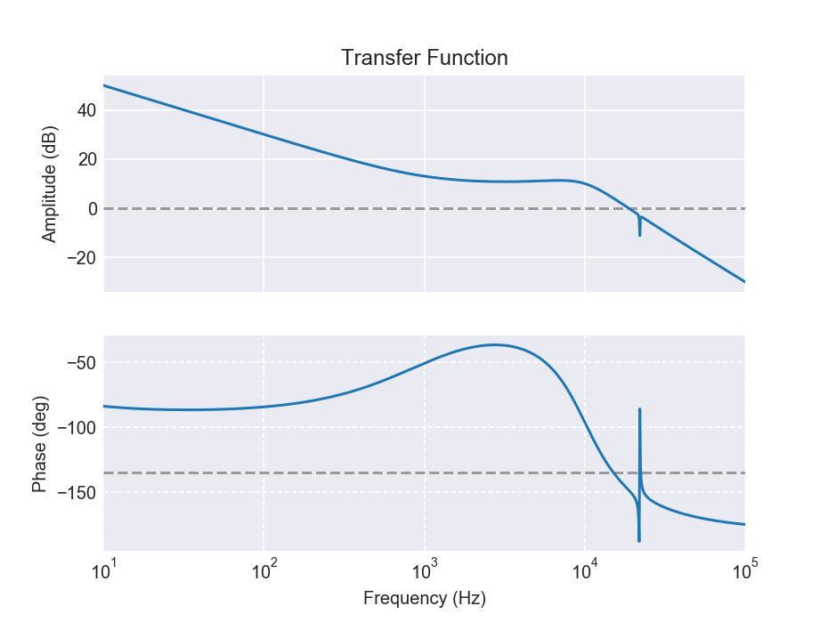
The servo can be applied to the measured transfer function of the system that is to be controlled (the plant):
>>> plant = io.read(['Amplitude.txt', 'Phase.txt'])
>>> S = servo_design.ServoDesign()
>>> S.plant = plant
>>> S.integrator(100).notch(15.3e3, 5).integrator(4e3).lowpass(5e3, Q=0.5).notch(8.05e3, 10).gain(35)
                     zeros                      poles                                      gain
-------------------  -------------------------  -------------------------------------  --------
Gain                 []                         []                                     56.2341
Int 100Hz            [-100]                     [-0.1]                                  1
Notch 15.3kHz, Q=5   [ 0.+15300.j -0.-15300.j]  [-1530.+15223.308j -1530.-15223.308j]   1
Int 4kHz             [-4000.]                   [-4.]                                   1
LP2 5kHz, Q=0.5      []                         [-5000. -5000.]                         2.5e+07
Notch 8.05kHz, Q=10  [ 0.+8050.j -0.-8050.j]    [-402.5+8039.931j -402.5-8039.931j]     1
>>> S.plot()
which will show you the transfer function of the servo by its own (blue), and the combined open-loop gain of servo and plant (orange):
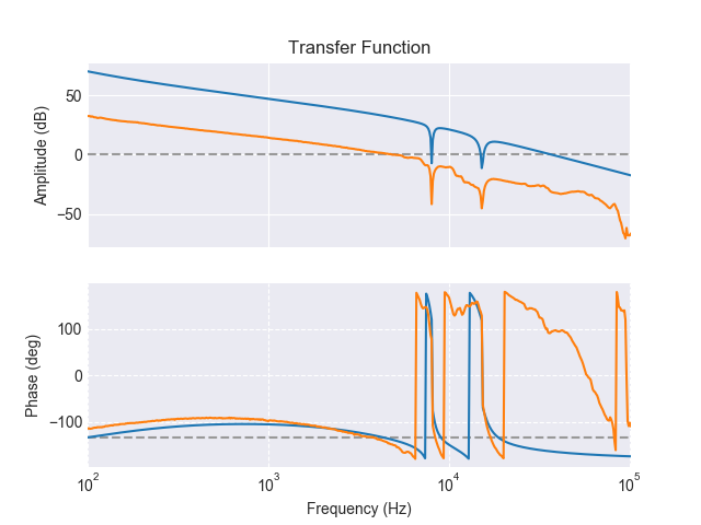
The grey dashed lines indicate unity gain (0dB) and a phase lag of 135deg, respectively, and can be used to hand-optimize phase and gain margin of the combined system.