Plotting traces from Spectrum Analyzer

Here’s how to import squeezing traces from a spectrum analyzer and plot them:

>>> %pylab inline
>>> from openqlab import *
>>> data = io.read(['vac.txt', 'sqz.txt', 'mcd.txt'])
>>> data.head()
                vac        sqz        mcd
Time (s)
0.000000 -58.208286 -60.882175 -47.536293
0.000321 -58.154301 -60.932739 -47.372425
0.000641 -58.077641 -60.914585 -47.569092
0.000962 -58.031555 -61.082169 -47.447727
0.001282 -58.066139 -60.975998 -47.460426
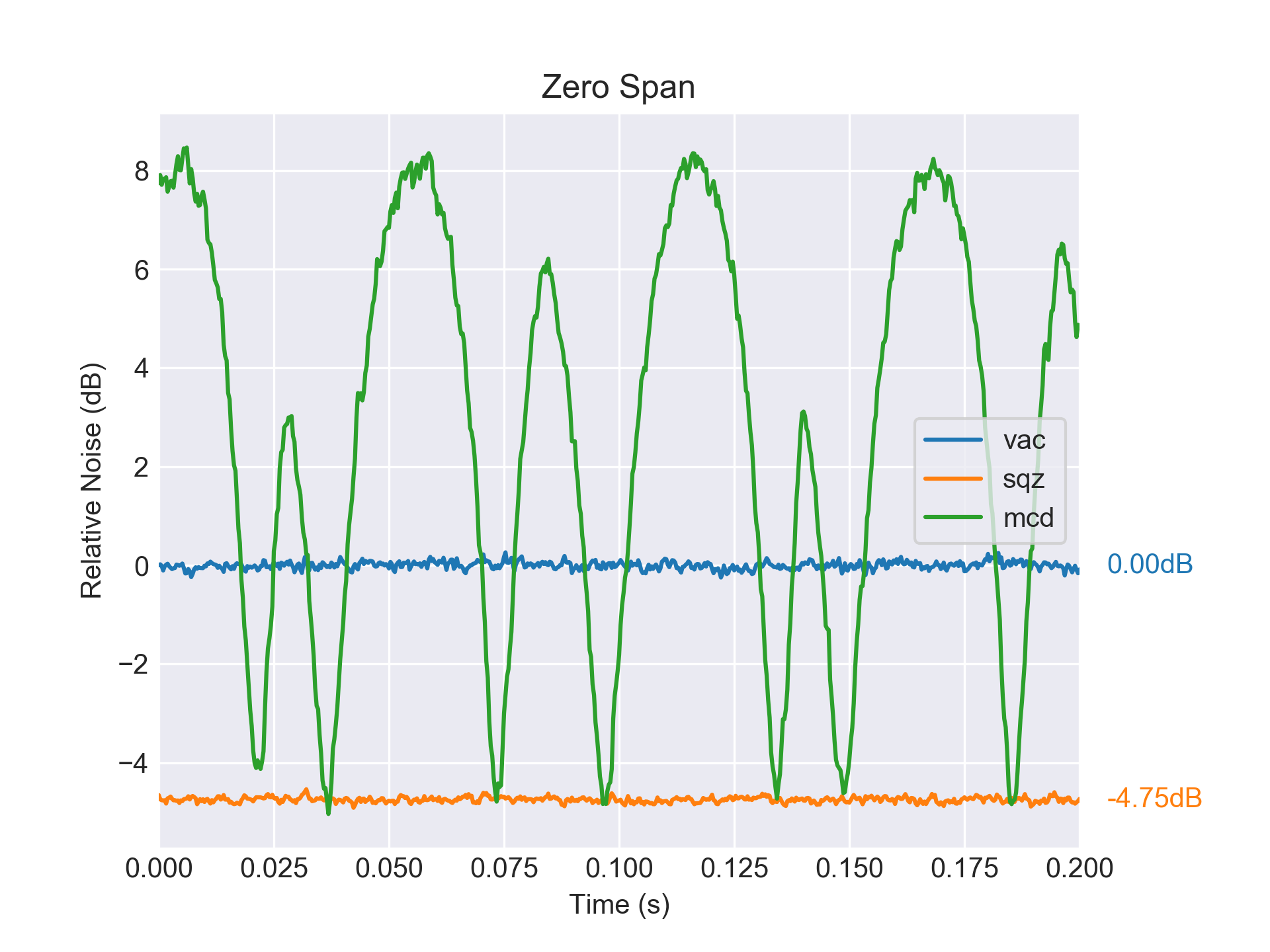
>>> fig = plots.zero_span(data)
< figure will be shown here when you have pylab inline enabled >
>>> fig.savefig('zero_span.pdf')

The figure will look something like this:

For a list of available plotting styles (e.g. Bode plots), have a look at openqlab.plots – Plotting of Data.

Some common file formats can be automatically recognized, e.g. Rhode & Schwarz spectrum analyzer data. In this case, the above call to io.read() works without specifying a file type. Some formats, however, cannot be recognized automatically and you will need to specify it explicitly:

>>> data = io.read(['Amplitude.txt'], type='flipper')

For a list of supported file formats and help on which of these can be automatically recognized, run

>>> io.list_formats()
< a list of currently supported formats will be shown here >